The Recamán Sequence
Computing the Recamán Sequence
The Recamán sequence is a fascinating integer sequence. It is in the OEIS as A005132; in fact its first terms spiral around the outside of the OEIS logo. It features in the Numberphile video The Slightly Spooky Recamán Sequence. It has inspired some beautiful artwork, and is discussed in many places on the internet.
I first heard of this sequence in a talk by Neil Sloane in 2006, and I have returned to it many times over the years, through many generations of computing hardware and compilers. Altogether I’ve probably invested more time and energy in this project than almost any other.
The definition is simple: the first term, a(0), is 0. Then to get the nth term, we subtract n from the previous term, if the result would be non-negative and has not already appeared in the sequence; otherwise, we add n to the previous term. (Duplicate terms are allowed when adding.) So to get the first few terms:
- For a(1), we try subtracting 1 from a(0)=0, but that’s negative, so instead we add to get a(1) = 1.
- For a(2), we try subtracting 2 from a(1)=1, but that’s negative, so we add to get a(2) = 3.
- For a(3), we try subtracting 3 from a(2)=3, but 0 has already appeared at a(0), so we add to get a(3) = 6.
- For a(4), we try subtracting 4 from a(3)=6, and this time it works: 2 is positive and has not already appeared, so a(4) = 2.
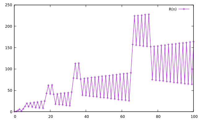
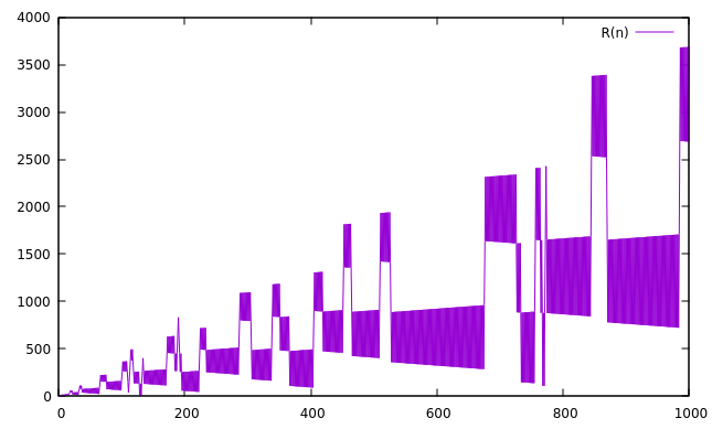
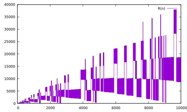
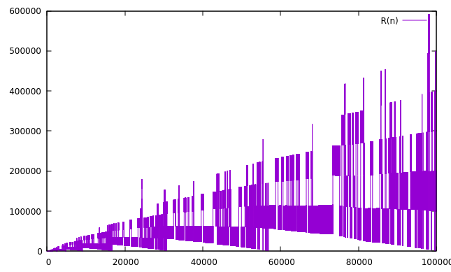
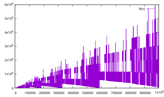
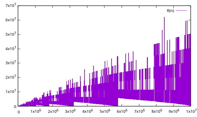
Below are graphs of the initial 102 to 107 terms:
Questions
Some interesting questions we can try to approach computationally are:
- Does every non-negative value eventually appear in the sequence?
- What numbers have not yet appeared, and what are the terms where it fills in the smallest missing number? (Spoiler alert: see A064227.)
- Where does the sequence reach a new record height (addition steps minus subtraction steps)? (A064292)
- What terms set new records for the most addition or subtraction steps in a row?
Terms can only be small relative to n when (a(n) mod n) is small – if the terms are close to (but larger than) a multiple of n, we might be able to subtract away most of the value of the previous term, leaving only a small remainder. The value of (a(n) mod n) stays the same or decreases from one term to the next, until it “wraps around” to a value close to n (see A065052). The smallest term seen since the last wraparound is a local minimum, or landing. Landings are the terminal points of the downward arcs seen in the graphs above, such as a(403)=92 and a(4971)=426, and are the places where the sequence has a chance to fill in a missing small number. The locations and values of these landings have not previously been recorded in the OEIS.
Results
I computed the Recamán sequence to over 10612 terms, over a period of about 14 months on an Intel Skylake-generation system with 256GB of memory and a 30TB disk array. See below for details on the algorithm.
Here is a plot of the first 10612 terms, with log scale (base 10) on both axes. The overall slope of the graph is about 16.
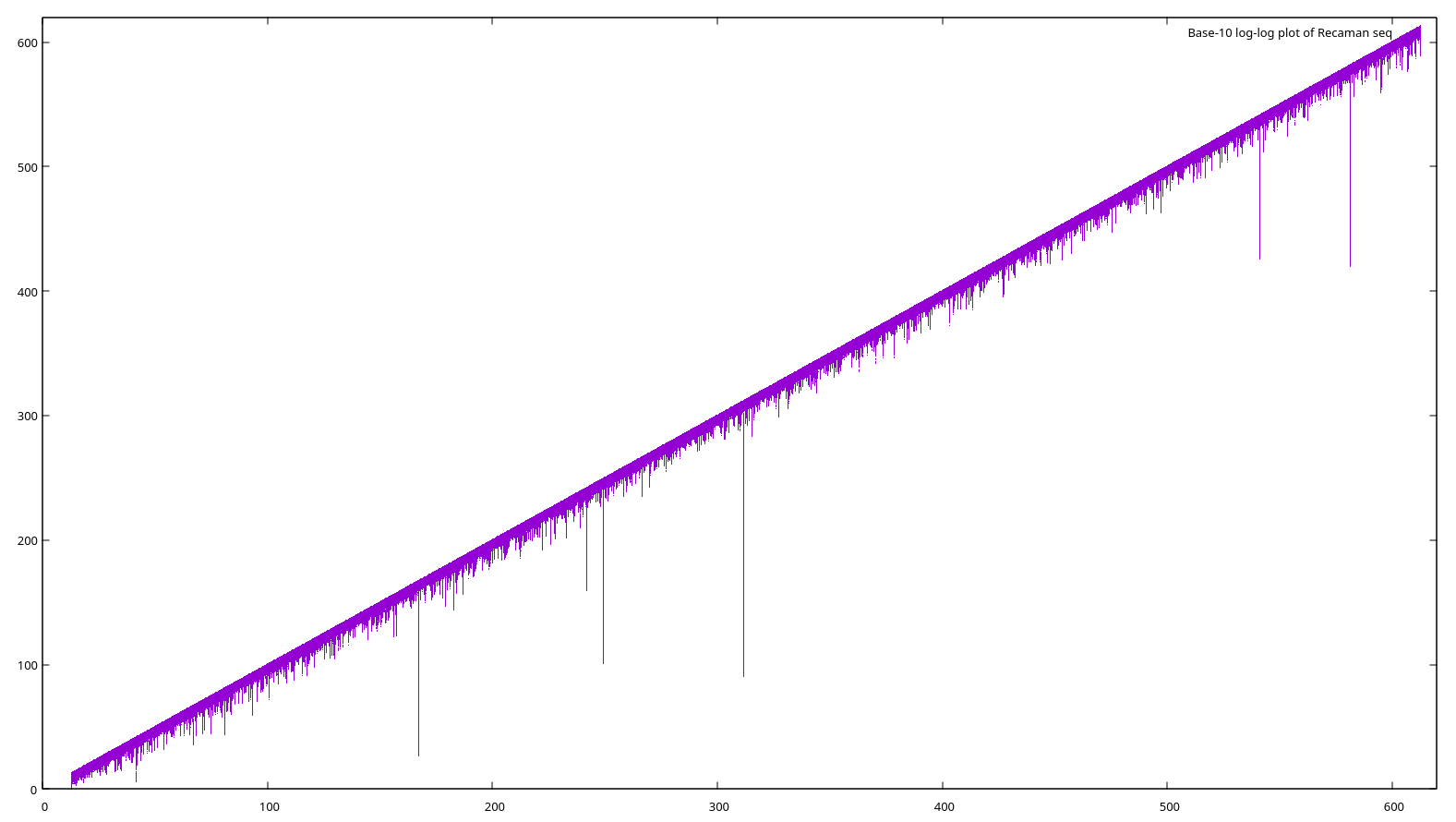
Each of the little downward spikes (and many more too small or close together to see) is a landing. There are several near misses, where the sequence gets quite low without filling the bottom-most hole. The lowest it goes after hitting 2406 is a(899989616955022684) = 963744. The most dramatic is around term 1041, at a(177900612666336352118510768792480139301821) = 2023155. After that, the lowest it gets is about 1027, around term 10167. And after 10612 terms, 852655 remains the smallest missing number.
Full results:
- All landings up to 10612 terms (see new sequences A393814 and A393815)
- All holes less than 232, after 10612 terms
- Terms which set or tie a record number of addition steps or subtraction steps (see new sequences A390717 and A392407)
- Terms with maximum height (see A064292 and A064290)
Computation
Computing terms of the sequence one by one is easy, just following the rule above. But we can go faster: in the graphs above we can see that the sequence tends to alternate addition and subtraction, ping-ponging between two ranges of consecutive numbers (see A119632). For example, terms a(6) - a(17) are: 13, 20, 12, 21, 11, 22, 10, 23, 9, 24, 8, 25; these form a lower range of 13 down to 8, and an upper range of 20 up to 25. In general, this ping-pong pattern will continue until one of two things happens:
- The lower range bumps into a number which has already appeared in the sequence, so we can’t subtract; then we add twice in a row
- The lower range passes over a “hole” farther down which allows us to subtract twice in a row
At the beginning of a ping-pong section, we can look ahead to find the which of these two terminal conditions will happen first and in how many steps, and then we know that all the intervening terms form two contiguous ranges, without having to compute them individually. In practice, the ping-pong sections get exponentially longer as the sequence progresses, so the computation also accelerates. In the graphs above, each trapezoidal block is generally a ping-pong section which can be computed in a single step of this algorithm.
Detecting condition #1 is relatively easy; we just look for the closest number below the lower range which is already taken. Condition #2 is more complicated, because only every third number is tested. Using the same example as above, a(6)=13; to get a(7) we try 13-7=6, which has already appeared. In this case 6 was the potential “hole” which would have allowed us to subtract twice in a row. Now a(8)=12, and to get a(9) we try 12-9=3; 3 is the potential “hole”. So to detect condition #2 we need to find the first lower untaken number which is a multiple of 3 steps away.
All that takes a little fiddling to get right, but the real kicker is the part about whether a number has already appeared in the sequence: you have to remember its entire history, and be able to refer back to it constantly! From here on, it’s all about how to efficiently store and compute with these vast quantities of data.
Little big numbers
We’re going to be getting into some pretty big numbers. There are plenty of libraries like GMP which handle arbitrary-precision integers, but their numbers are typically implemented as a data structure which has a storage array of 64-bit elements for the data, and some additional fields containing other information about the number, like its size. Also the storage array may be dynamically allocated, which means there is additional metadata maintained by the malloc library. The numbers of this sequence are big-ish, but not that big – up to a couple hundred bytes – so that overhead is significant. I want to store as many numbers as possible as densely as possible, without any space wasted on metadata or padding out to a multiple of 64 bits.
There’s always a price to be paid somewhere. My solution is extremely space-efficient, not too bad for performance, and terrible for complexity and code size. I use C++ templates to create a different class for numbers of each different size in bytes. The operators for addition, comparison, etc. are overridden to work on arbitrary-sized arrays of bytes, and the class is declared with __attribute__ ((packed)) so that arrays of them will not be padded to get nice data alignment.
I went through many versions of C code, inline assembly, and compiler intrinsics over the years to try to get these to use well-performing code. Most recently, I found that the clang compiler can recognize a specific code pattern as being a multi-precision add or subtract. So the routine for the += operator looks like this, where n is an array of bytes, b is the template parameter which is the length of n, and U64, U32 and U16 are macros which cast the argument to be a 64/32/16-bit pointer and dereference it:
inline varnum<b>& operator += (const varnum<b> &x)
{
    int64_t carry=0;

    // Add all the full 8-byte chunks of x to this. The code uses 128-bit math to add the two
    // sources plus carry-in and then extracts the carry-out from the upper 64 bits of the result,
    // but the compiler should turn this into an efficient sequence of add-carry instructions.
    for (int i=0; i<=b-8; i+=8) {
        int128_t temp = (int128_t)carry + U64(n+i) + U64(x.n+i);
        U64(n+i) = temp;
        carry = temp >> 64;
    }

    // Add any remaining upper bytes using 4/2/1-byte instructions
    if (b & 0x4) {
        int64_t temp = (int64_t)carry + U32(n+(b&(~0x7))) + U32(x.n+(b&(~0x7)));
        U32(n+(b&(~0x7))) = temp;
        carry = temp >> 32;
    }
    if (b & 0x2) {
        int32_t temp = (int32_t)carry + U16(n+(b&(~0x3))) + U16(x.n+(b&(~0x3)));
        U16(n+(b&(~0x3))) = temp;
        carry = temp >> 16;
    }
    if (b & 0x1)
        n[b-1] = carry + n[b-1] + x.n[b-1];

    return *this;
}
Since b is known at compile time, this produces the optimal sequence of add-carry instructions: as many 64-bit add-carrys as needed, and maybe 32/16/8-bit add-carrys to finish off the bytes at the top, if needed depending on the size of the number.
Similar routines implement other basic operations like assignment, arithmetic, and comparison, with special cases for some common things like comparison to zero and comparison to x +/- 1. For div and mod by 3, I just convert to a GMP integer and use the library routines.
Storing ranges
Since the sequence naturally contains many sequences of sequential numbers, it’s much more efficent to store just the endpoints of ranges. A good structure for quickly adding and removing ordered things is a red-black tree. But a fast implementation of a red-black tree wants to store a bunch of stuff in each node, including pointers to its left and right children, parent, and next/previous nodes, which is a lot of storage overhead.
One trick to cut the size of the pointers in half is to allocate a large single storage array up front, and use 32-bit indices into it, instead of actual 64-bit pointers. But it’s still a lot of overhead. To amortize that cost, each node stores not just one range, but an array of ranges. The size of the array varies with the size of the numbers being stored in the tree, but is kept between 100 and 200. (The reason for not having a constant array size is explained below.)
The basic range_tree is templated on the size of the varnum numbers in its ranges, and supports several key operations:
- Adding a range: The new range may connect or overlap one or more ranges within a node, and/or span multiple nodes (which leads to so many special cases). If the new range combines with existing ranges then the node may end up with fewer valid ranges than it had before. If a new range needs to be inserted then the tail of the array is shifted over to make room; if the array is full then the last range is moved to a newly inserted node, making room to insert the new range.
- Querying whether a particular number is present in any of the ranges.
- Find the closest number lower than N which is taken. This is the check for case #1 in the fast computation.
- Find the closest number lower than N which is not taken and is a multiple of 3 away from N. This is the check for case #2.
- Garbage collection: over time the tree gets cluttered with underutilized nodes, which occur when ranges coalesce or when new nodes containing a single range are inserted. When the ratio of invalid ranges gets too high, the tree repacks all ranges into full nodes, and recycles all extra nodes back into a freelist. It then shuffles the nodes in the underlying storage array so that they are located at sequential addresses, which helps with memory locality and paging (below).
Overall, the base range_tree gives highly space-efficient storage for ranges of a specific number size, with reasonable performance; using appropriate choices for array size and garbage collection thresholds, less than 1% of storage is used for anything other than the actual, non-zero data bytes.
Variable-sized ranges
The next layer is the var_range_tree, which has an array of range_tree of each size. In fact, it’s advantageous to limit the size of any individual tree (for garbage collection; see paging section below), so I keep one tree for every bit size. I set the maximum number size to 2048 bits, so I have 2048 trees of ranges.
All the math in the main algorithm is done using max-sized numbers, which are the inputs to the var_range_tree functions. It determines the actual size in bits of the input number and passes the operation on to the appropriate tree. For the search functions (e.g. closest lower taken number), an individual tree may return that its search fell off the lower end of the tree, in which case the same query is made of the next smaller tree. All the var_range_tree functions track a bitmap of which trees have been accessed and/or modified, which is periodically output and reset – this is the source of the “paint-dripping” graphs above.
Paging
Now we have everything we need to compute the sequence quickly and store all the terms very densely in memory. With 240GB of RAM allocated to range storage, it runs for less than a day before running out of room, reaching roughly term 1053. To go further, we’ll need some secondary storage.
Within the range_tree, the node storage is divided into 64MB pages – the page size is chosen to balance storage and disk I/O granularity with the overhead of tracking data needed for each page. Every reference to a node first figures out which page the node is in; the number of nodes per page is always a power of 2 so that this can be done quickly with a shift. To avoid wasting space at the end of each page, the number of ranges per tree node is chosen differently for each tree size to ensure that a power of 2 nodes fits as tightly as possible in a page. (This has to be done with compile-time macros because the array size is a template parameter to the node, to avoid dynamic allocation of each range array.)
After computing the page number, a node reference checks whether the page is present in memory. If not, it chooses a victim page to swap out to disk, and brings in the needed page. Obviously the page replacement policy will matter a lot here, and the details of paging and its interaction with garbage collection needed many rounds of tuning to avoid thrashing. In particular, it’s a really bad idea to garbage collect a tree which is larger than RAM, as the reshuffling of nodes causes nearly endless swapping back and forth (this is why I use separate trees for each bit size, instead of byte size).
As described above, the high-level pattern of the sequence is that the upper (increasing) ranges continue to increase steadily, while the lower (decreasing) ranges decrease to some local minimum and then jump back up. This means that standard replacement policies like LRU (least recently used) don’t work well, because the lower ranges will walk through lots of data which is only briefly used. Instead, I keep a small number of recently used pages, and after that prefer those which store larger numbers. This means that when a downward arc completes, most of memory still contains data from the uppermost portions of the sequence, which will be useful.
Storage
For disk storage, I built an array of four 8TB hard drives. To maximize data transfer speed I used the btrfs filesystem to organize them as a RAID-0 array, where data is striped across all the drives, giving 4x the read and write bandwidth of a single drive. I also enabled automatic disk compression, which shrunk the data by about 26% on average. At the end of the computation, the disk held 36TB of uncompressed data. (Although my maximum 2048-bit varnum size ended up being the limit which ended the run, not disk space.)
For most of the life of this project I just hoped that everything would run for a long time without crashing or losing power, but eventually this proved too difficult and I had to implement checkpointing, where all the in-memory pages are flushed to disk, and all global data is saved away. This is a time-consuming process, so I triggered it manually every few weeks. After creating a checkpoint, I used btrfs snapshot to create a clone of the whole storage area; the files are copy-on-write so this costs no disk space until a file is modified.
Correctness
With any complex, long-running computation, there are justifiable concerns about incorrect results, due either to program bugs or data corruption on disk, in memory, or in the CPU itself.
As the program runs, it prints out the current term at exponentially increasing intervals. Over the course of the whole run, this produces several gigabytes of sort-of-randomly chosen terms. As the program has evolved over time, every run of a new version has its output compared against previous versions. Because of the iterative nature of the computation, bugs (at least the ones I have found and fixed, of course) have generally manifested quickly as a divergence from the expected output. The first 10230 terms at least have been run a number of times and always generated the same output, which makes both recently introduced bugs and data corruption unlikely. The final portion of the maximal computation has only been run once.
As a further guard against silent memory corruption, on every garbage collection the contents of the tree are checked for consistency – that the start and end of each range are in the correct order with respect to each other and to the previous and next ranges. Of course this can’t detect all errors, but experiments with introducing random single-bit errors found that it detected them with a high probability.
For data stored on disk, btrfs does automatic checksumming of all data, which should detect corruption. (It cannot correct errors, so if the checksum fails I would still have to revert to the previous checkpoint.) Many pages are unmodified for a long time, and so persist across several checkpoints, so on every checkpoint I also computed the MD5 sum of each page and compared it to the previous checkpoint to ensure that there were no changes in unexpected pages.
None of that is bulletproof, of course – my program could still have longstanding or corner-case bugs, or there could have been undetected data corruption. But overall I have reasonable confidence in the results.